4.1. SciPy - Librairie d’algorithmes pour le calcul scientifique en Python
Librairie de calcul numérique : intégration numérique, résolution d’équations différentielles, algèbre linéaire, traitement du signal, optimisation…
 #Pour intégrer les graphes à votre notebook, il suffit de faire
%matplotlib inline
from jyquickhelper import add_notebook_menu
add_notebook_menu()
4.1.1. Introduction
SciPy s’appuie sur NumPy.
SciPy fournit des implémentations efficaces d’algorithmes standards.
Certains des sujets couverts par SciPy:
Fonctions Spéciales (scipy.special)
Intégration (scipy.integrate)
Optimisation (scipy.optimize)
Interpolation (scipy.interpolate)
Transformées de Fourier (scipy.fftpack)
Traitement du Signal (scipy.signal)
Algèbre Linéaire (scipy.linalg)
Matrices Sparses et Algèbre Linéaire Sparse (scipy.sparse)
Statistiques (scipy.stats)
Traitement d’images N-dimensionelles (scipy.ndimage)
Lecture/Ecriture Fichiers IO (scipy.io)
Durant ce cours on abordera certains de ces modules.
Pour utiliser un module de SciPy dans un programme Python il faut commencer par l’importer.
Voici un exemple avec le module linalg
from scipy import linalg
On aura besoin de NumPy:
import numpy as np
Et de matplotlib/pylab:
# et JUSTE POUR MOI (pour avoir les figures dans le notebook)
%matplotlib inline
import matplotlib.pyplot as plt
4.1.2. Fonctions Spéciales
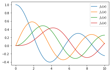
Un grand nombre de fonctions importantes, notamment en physique, sont disponibles dans le module scipy.special
Pour plus de détails: http://docs.scipy.org/doc/scipy/reference/special.html#module-scipy.special.
Un exemple avec les fonctions de Bessel:
# jn : Bessel de premier type
# yn : Bessel de deuxième type
from scipy.special import jn, yn
jn?
n = 0    # ordre
x = 0.0

# Bessel de premier type
print ("J_%d(%s) = %f" % (n, x, jn(n, x)))

x = 1.0
# Bessel de deuxième type
print("Y_%d(%s) = %f" % (n, x, yn(n, x)))
J_0(0.0) = 1.000000
Y_0(1.0) = 0.088257
x = np.linspace(0, 10, 100)

for n in range(4):
    plt.plot(x, jn(n, x), label=r"$J_%d(x)$" % n)
plt.legend()
<matplotlib.legend.Legend at 0x11e549fa0>
from scipy import special
special?
4.1.3. Intégration
4.1.3.1. intégration numerique
L’évaluation numérique de:
\(\displaystyle \int_a^b f(x) dx\)
est nommée quadrature (abbr. quad). SciPy fournit différentes fonctions: par exemple quad, dblquad et tplquad pour les intégrales simples, doubles ou triples.
from scipy.integrate import quad, dblquad, tplquad
quad?
L’usage de base:
# soit une fonction f
def f(x):
    return x
a, b = 1, 2 # intégrale entre a et b

val, abserr = quad(f, a, b)

print ("intégrale =", val, ", erreur =", abserr )
intégrale = 1.5 , erreur = 1.6653345369377348e-14
Exemple intégrale double:
\(\int_{x=1}^{2} \int_{y=1}^{x} (x + y^2) dx dy\)
dblquad?
def f(y, x):
    return x + y**2

def gfun(x):
    return 1

def hfun(x):
    return x

print(dblquad(f, 1, 2, gfun, hfun))
(1.7500000000000002, 4.7941068289487755e-14)
4.1.3.2. Equations différentielles ordinaires (EDO)
SciPy fournit deux façons de résoudre les EDO: Une API basée sur la fonction odeint, et une API orientée-objet basée sur la classe ode.
odeint est plus simple pour commencer.
Commençons par l’importer:
from scipy.integrate import odeint
Un système d’EDO se formule de la façon standard:
\(y' = f(y, t)\)
avec
\(y = [y_1(t), y_2(t), ..., y_n(t)]\)
et \(f\) est une fonction qui fournit les dérivées des fonctions \(y_i(t)\). Pour résoudre une EDO il faut spécifier \(f\) et les conditions initiales, \(y(0)\).
Une fois définies, on peut utiliser odeint:
y_t = odeint(f, y_0, t)
où t est un NumPy array des coordonnées en temps où résoudre l’EDO. y_t est un array avec une ligne pour chaque point du temps t, et chaque colonne correspond à la solution y_i(t) à chaque point du temps.
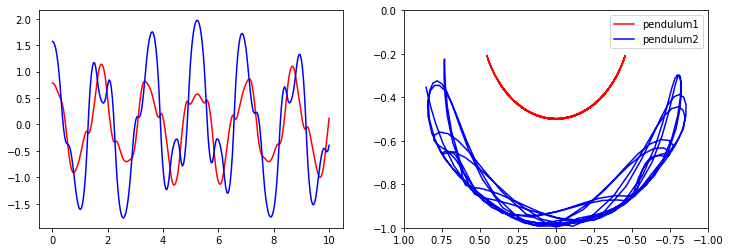
4.1.3.2.1. Exemple: double pendule
Description: http://en.wikipedia.org/wiki/Double_pendulum
from IPython.core.display import Image
Image(url='http://upload.wikimedia.org/wikipedia/commons/c/c9/Double-compound-pendulum-dimensioned.svg')

Les équations du mouvement du pendule sont données sur la page wikipedia:
\({\dot \theta_1} = \frac{6}{m\ell^2} \frac{ 2 p_{\theta_1} - 3 \cos(\theta_1-\theta_2) p_{\theta_2}}{16 - 9 \cos^2(\theta_1-\theta_2)}\)
\({\dot \theta_2} = \frac{6}{m\ell^2} \frac{ 8 p_{\theta_2} - 3 \cos(\theta_1-\theta_2) p_{\theta_1}}{16 - 9 \cos^2(\theta_1-\theta_2)}.\)
\({\dot p_{\theta_1}} = -\frac{1}{2} m \ell^2 \left [ {\dot \theta_1} {\dot \theta_2} \sin (\theta_1-\theta_2) + 3 \frac{g}{\ell} \sin \theta_1 \right ]\)
\({\dot p_{\theta_2}} = -\frac{1}{2} m \ell^2 \left [ -{\dot \theta_1} {\dot \theta_2} \sin (\theta_1-\theta_2) + \frac{g}{\ell} \sin \theta_2 \right]\)
où les \(p_{\theta_i}\) sont les moments d’inertie. Pour simplifier le code Python, on peut introduire la variable \(x = [\theta_1, \theta_2, p_{\theta_1}, p_{\theta_2}]\)
\({\dot x_1} = \frac{6}{m\ell^2} \frac{ 2 x_3 - 3 \cos(x_1-x_2) x_4}{16 - 9 \cos^2(x_1-x_2)}\)
\({\dot x_2} = \frac{6}{m\ell^2} \frac{ 8 x_4 - 3 \cos(x_1-x_2) x_3}{16 - 9 \cos^2(x_1-x_2)}\)
\({\dot x_3} = -\frac{1}{2} m \ell^2 \left [ {\dot x_1} {\dot x_2} \sin (x_1-x_2) + 3 \frac{g}{\ell} \sin x_1 \right ]\)
\({\dot x_4} = -\frac{1}{2} m \ell^2 \left [ -{\dot x_1} {\dot x_2} \sin (x_1-x_2) + \frac{g}{\ell} \sin x_2 \right]\)
g = 9.82
L = 0.5
m = 0.1

def dx(x, t):
    """The right-hand side of the pendulum ODE"""
    x1, x2, x3, x4 = x[0], x[1], x[2], x[3]

    dx1 = 6.0/(m*L**2) * (2 * x3 - 3 * np.cos(x1-x2) * x4)/(16 - 9 * np.cos(x1-x2)**2)
    dx2 = 6.0/(m*L**2) * (8 * x4 - 3 * np.cos(x1-x2) * x3)/(16 - 9 * np.cos(x1-x2)**2)
    dx3 = -0.5 * m * L**2 * ( dx1 * dx2 * np.sin(x1-x2) + 3 * (g/L) * np.sin(x1))
    dx4 = -0.5 * m * L**2 * (-dx1 * dx2 * np.sin(x1-x2) + (g/L) * np.sin(x2))

    return [dx1, dx2, dx3, dx4]
# on choisit une condition initiale
x0 = [np.pi/4, np.pi/2, 0, 0]
# les instants du temps: de 0 à 10 secondes
t = np.linspace(0, 10, 250)
# On résout
x = odeint(dx, x0, t)
print(x.shape)
(250, 4)
# affichage des angles en fonction du temps
fig, axes = plt.subplots(1,2, figsize=(12,4))
axes[0].plot(t, x[:, 0], 'r', label="theta1")
axes[0].plot(t, x[:, 1], 'b', label="theta2")

x1 = + L * np.sin(x[:, 0])
y1 = - L * np.cos(x[:, 0])
x2 = x1 + L * np.sin(x[:, 1])
y2 = y1 - L * np.cos(x[:, 1])

axes[1].plot(x1, y1, 'r', label="pendulum1")
axes[1].plot(x2, y2, 'b', label="pendulum2")
axes[1].set_ylim([-1, 0])
axes[1].set_xlim([1, -1])
plt.legend()
<matplotlib.legend.Legend at 0x11f36d8b0>
4.1.4. Transformées de Fourier
SciPy utilise la librairie FFTPACK écrite en FORTRAN.
Commençons par l’import:
from scipy import fftpack
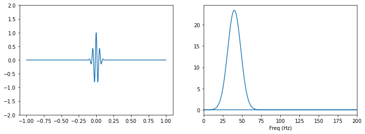
Nous allons calculer les transformées de Fourier discrètes de fonctions spéciales:
from scipy.signal import gausspulse

t = np.linspace(-1, 1, 1000)
x = gausspulse(t, fc=20, bw=0.5)

# Calcul de la TFD
F = fftpack.fft(x)

# calcul des fréquences en Hz si on suppose un échantillonage à 1000Hz
freqs = fftpack.fftfreq(len(x), 1. / 1000.)
fig, axes = plt.subplots(1, 2, figsize=(12,4))
axes[0].plot(t, x) # plot du signal
axes[0].set_ylim([-2, 2])

axes[1].plot(freqs, np.abs(F)) # plot du module de la TFD
axes[1].set_xlim([0, 200])
# mask = (freqs > 0) & (freqs < 200)
# axes[0].plot(freqs[mask], abs(F[mask])) # plot du module de la TFD
axes[1].set_xlabel('Freq (Hz)')
plt.show()
4.1.5. Algèbre linéaire
Le module de SciPy pour l’algèbre linéaire est linalg. Il inclut des routines pour la résolution des systèmes linéaires, recherche de vecteur/valeurs propres, SVD, Pivot de Gauss (LU, cholesky), calcul de déterminant etc.
Documentation : http://docs.scipy.org/doc/scipy/reference/linalg.html
4.1.5.1. Résolution d’equations linéaires
Trouver x tel que:
\(A x = b\)
avec \(A\) une matrice et \(x,b\) des vecteurs.
A = np.array([[1,0,3], [4,5,12], [7,8,9]], dtype=np.float)
b = np.array([[1,2,3]], dtype=np.float).T
print (A)
print (b)
[[ 1.  0.  3.]
 [ 4.  5. 12.]
 [ 7.  8.  9.]]
[[1.]
 [2.]
 [3.]]
/var/folders/2b/cj2pm60x61s5qlxpmr7g7km00000gn/T/ipykernel_6824/4101427969.py:1: DeprecationWarning: `np.float` is a deprecated alias for the builtin `float`. To silence this warning, use `float` by itself. Doing this will not modify any behavior and is safe. If you specifically wanted the numpy scalar type, use `np.float64` here.
Deprecated in NumPy 1.20; for more details and guidance: https://numpy.org/devdocs/release/1.20.0-notes.html#deprecations
  A = np.array([[1,0,3], [4,5,12], [7,8,9]], dtype=np.float)
/var/folders/2b/cj2pm60x61s5qlxpmr7g7km00000gn/T/ipykernel_6824/4101427969.py:2: DeprecationWarning: `np.float` is a deprecated alias for the builtin `float`. To silence this warning, use `float` by itself. Doing this will not modify any behavior and is safe. If you specifically wanted the numpy scalar type, use `np.float64` here.
Deprecated in NumPy 1.20; for more details and guidance: https://numpy.org/devdocs/release/1.20.0-notes.html#deprecations
  b = np.array([[1,2,3]], dtype=np.float).T
from scipy import linalg
x = linalg.solve(A, b)
print (x)
[[ 0.8       ]
 [-0.4       ]
 [ 0.06666667]]
print (x.shape)
print (b.shape)
(3, 1)
(3, 1)
4.1.5.2. Valeurs propres et vecteurs propres
\(\displaystyle A v_n = \lambda_n v_n\)
avec \(v_n\) le \(n\)ème vecteur propre et \(\lambda_n\) la \(n\)ème valeur propre.
Les fonctions sont: eigvals et eig
A = np.random.randn(3, 3)
evals, evecs = linalg.eig(A)
evals
array([0.91414406+1.81276219j, 0.91414406-1.81276219j,
       0.76157097+0.j        ])
evecs
array([[ 0.2128791 -0.43107519j,  0.2128791 +0.43107519j,
        -0.52670265+0.j        ],
       [ 0.25367591+0.26548999j,  0.25367591-0.26548999j,
        -0.5012345 +0.j        ],
       [ 0.7962539 +0.j        ,  0.7962539 -0.j        ,
         0.6865481 +0.j        ]])
Si A est symmétrique
A = A + A.T
# A += A.T  # ATTENTION MARCHE PAS !!!!
evals = linalg.eigvalsh(A)
print (evals)
[-0.54075499 1.81508054 3.90539263]
print (linalg.eigh(A))
(array([-0.54075499,  1.81508054,  3.90539263]), array([[ 0.531646  ,  0.78940516, -0.30690718],
       [-0.45772314,  0.57267589,  0.68009694],
       [ 0.71263038, -0.2210923 ,  0.66578986]]))
4.1.5.3. Opérations matricielles
# inversion
linalg.inv(A)
array([[-0.15524812,  0.64563222, -0.84910387],
       [ 0.64563222, -0.0883216 ,  0.64939326],
       [-0.84910387,  0.64939326, -0.7987007 ]])
# vérifier
# déterminant
linalg.det(A)
-3.8331969491783897
# normes
print (linalg.norm(A, ord='fro'))  # frobenius
print (linalg.norm(A, ord=2))
print (linalg.norm(A, ord=np.inf))
4.340394552237356
3.905392625491531
4.579888196899612
4.1.6. Optimisation
Objectif: trouver les minima ou maxima d’une fonction
Doc : http://scipy-lectures.github.com/advanced/mathematical_optimization/index.html
On commence par l’import
from scipy import optimize
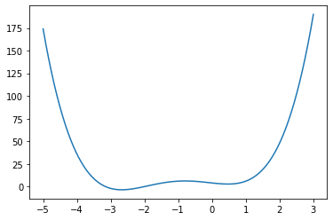
4.1.6.1. Trouver un minimum
def f(x):
    return 4*x**3 + (x-2)**2 + x**4
x = np.linspace(-5, 3, 100)
plt.plot(x, f(x))
[<matplotlib.lines.Line2D at 0x1203c69a0>]
Nous allons utiliser la fonction fmin_bfgs:
x_min = optimize.fmin_bfgs(f, x0=-3)
x_min
Optimization terminated successfully.
         Current function value: -3.506641
         Iterations: 4
         Function evaluations: 12
         Gradient evaluations: 6
array([-2.67298165])
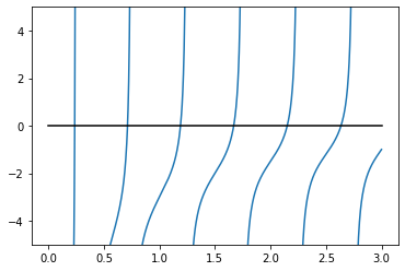
4.1.6.2. Trouver les zéros d’une fonction
Trouver \(x\) tel que \(f(x) = 0\). On va utiliser fsolve.
omega_c = 3.0
def f(omega):
    return np.tan(2*np.pi*omega) - omega_c/omega
x = np.linspace(0, 3, 1000)
y = f(x)
mask = np.where(abs(y) > 50)
x[mask] = y[mask] = np.nan # get rid of vertical line when the function flip sign
plt.plot(x, y)
plt.plot([0, 3], [0, 0], 'k')
plt.ylim(-5,5)
/var/folders/2b/cj2pm60x61s5qlxpmr7g7km00000gn/T/ipykernel_6824/2455056392.py:3: RuntimeWarning: divide by zero encountered in true_divide
  return np.tan(2*np.pi*omega) - omega_c/omega
(-5.0, 5.0)
np.unique(
    (optimize.fsolve(f, np.linspace(0.2, 3, 40))*1000).astype(int)
) / 1000.
array([0.237, 0.712, 1.189, 1.669, 2.15 , 2.635, 3.121, 3.61 ])
optimize.fsolve(f, 0.72)
array([0.71286972])
optimize.fsolve(f, 1.1)
array([1.18990285])
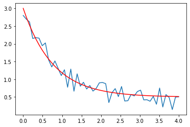
4.1.6.2.1. Estimation de paramètres de fonctions
from scipy.optimize import curve_fit

def f(x, a, b, c):
    """
    f(x) = a exp(-bx) + c
    """
    return a*np.exp(-b*x) + c

x = np.linspace(0, 4, 50)
y = f(x, 2.5, 1.3, 0.5)
yn = y + 0.2*np.random.randn(len(x))  # ajout de bruit
plt.plot(x, yn)
plt.plot(x, y, 'r')
[<matplotlib.lines.Line2D at 0x1204fff10>]
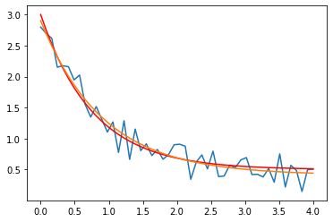
(a, b, c), _ = curve_fit(f, x, yn)
print (a, b, c)
2.488415266050443 1.0927540556794324 0.41113802241565106
curve_fit?
On affiche la fonction estimée:
plt.plot(x, yn)
plt.plot(x, y, 'r')
plt.plot(x, f(x, a, b, c))
[<matplotlib.lines.Line2D at 0x1205e39d0>]
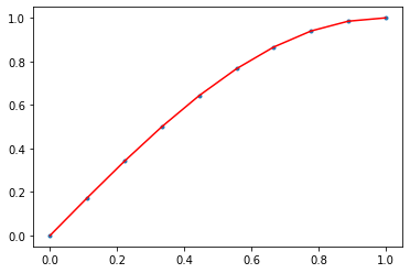
Dans le cas de polynôme on peut le faire directement avec NumPy
x = np.linspace(0,1,10)
y = np.sin(x * np.pi / 2.)
line = np.polyfit(x, y, deg=10)
plt.plot(x, y, '.')
plt.plot(x, np.polyval(line,x), 'r')
# xx = np.linspace(-5,4,100)
# plt.plot(xx, np.polyval(line,xx), 'g')
/opt/anaconda3/lib/python3.8/site-packages/IPython/core/interactiveshell.py:3457: RankWarning: Polyfit may be poorly conditioned
  exec(code_obj, self.user_global_ns, self.user_ns)
[<matplotlib.lines.Line2D at 0x120536f70>]
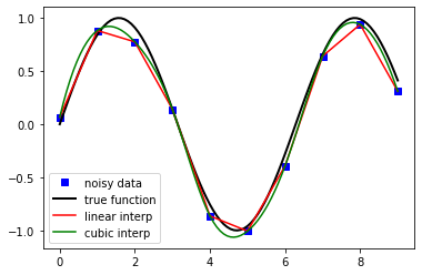
4.1.7. Interpolation
from scipy.interpolate import interp1d
def f(x):
    return np.sin(x)
n = np.arange(0, 10)
x = np.linspace(0, 9, 100)

y_meas = f(n) + 0.1 * np.random.randn(len(n)) # ajout de bruit
y_real = f(x)

linear_interpolation = interp1d(n, y_meas)
y_interp1 = linear_interpolation(x)

cubic_interpolation = interp1d(n, y_meas, kind='cubic')
y_interp2 = cubic_interpolation(x)
from scipy.interpolate import barycentric_interpolate, BarycentricInterpolator
BarycentricInterpolator??
plt.plot(n, y_meas, 'bs', label='noisy data')
plt.plot(x, y_real, 'k', lw=2, label='true function')
plt.plot(x, y_interp1, 'r', label='linear interp')
plt.plot(x, y_interp2, 'g', label='cubic interp')
plt.legend(loc=3);
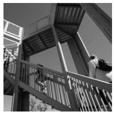
4.1.7.1. Images
from scipy import ndimage
from scipy import misc
img = misc.ascent()
print (img)
type(img), img.dtype, img.ndim, img.shape
[[ 83  83  83 ... 117 117 117]
 [ 82  82  83 ... 117 117 117]
 [ 80  81  83 ... 117 117 117]
 ...
 [178 178 178 ...  57  59  57]
 [178 178 178 ...  56  57  57]
 [178 178 178 ...  57  57  58]]
(numpy.ndarray, dtype('int64'), 2, (512, 512))
plt.imshow(img, cmap=plt.cm.gray)
plt.axis('off')
plt.show()
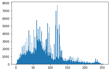
_ = plt.hist(img.reshape(img.size),200)
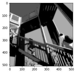
img[img < 70] = 50
img[(img >= 70) & (img < 110)] = 100
img[(img >= 110) & (img < 180)] = 150
img[(img >= 180)] = 200
plt.imshow(img, cmap=plt.cm.gray)
plt.axis('off')
plt.show()

Ajout d’un flou
img_flou = ndimage.gaussian_filter(img, sigma=2)
plt.imshow(img_flou, cmap=plt.cm.gray)
<matplotlib.image.AxesImage at 0x121136b80>
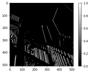
Application d’un filtre
img_sobel = ndimage.filters.sobel(img)
plt.imshow(np.abs(img_sobel) > 200, cmap=plt.cm.gray)
plt.colorbar()
<matplotlib.colorbar.Colorbar at 0x121cb9520>
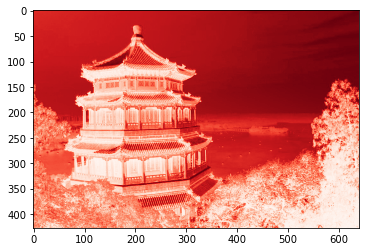
Accéder aux couches RGB d’une image:
import imageio
img = imageio.imread('china.jpg')
print (img.shape)
plt.imshow(img[:,:,0], cmap=plt.cm.Reds)
(427, 640, 3)
<matplotlib.image.AxesImage at 0x121f523a0>
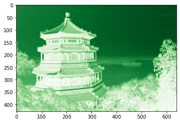
plt.imshow(img[:,:,1], cmap=plt.cm.Greens)
<matplotlib.image.AxesImage at 0x121ff47f0>
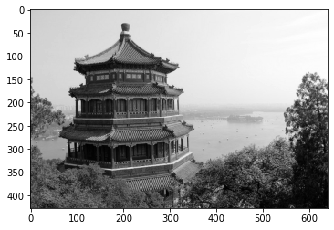
Conversion de l’image en niveaux de gris et affichage:
plt.imshow(np.mean(img, axis=2), cmap=plt.cm.gray)
<matplotlib.image.AxesImage at 0x120f39a00>
4.1.8. Pour aller plus loin
http://www.scipy.org - The official web page for the SciPy project.
http://docs.scipy.org/doc/scipy/reference/tutorial/index.html - A tutorial on how to get started using SciPy.